The Vorticity Cliff
A warp drive needs exotic matter — stuff with negative energy density that violates the laws of thermodynamics as we understand them. That’s been the deal since Miguel Alcubierre wrote the first equation in 1994. You want to move spacetime faster than light? Pay up in physics that doesn’t exist.
Except maybe it doesn’t have to be that way.
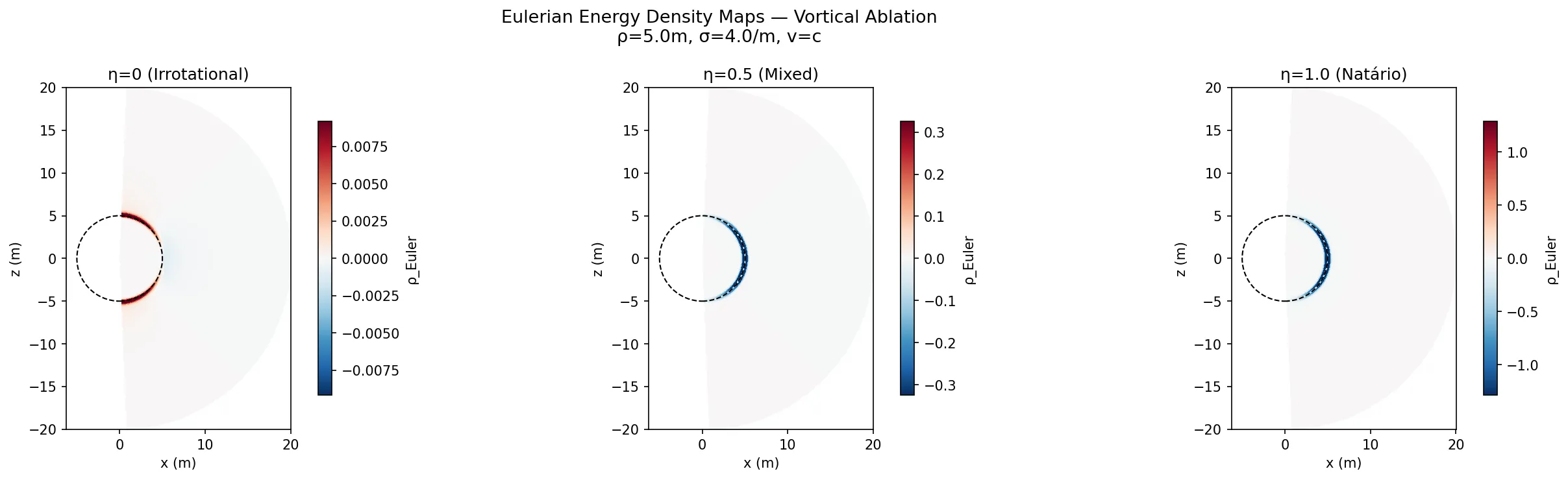 Energy density around three warp bubbles at the speed of light. Left: the irrotational Rodal metric — mostly positive (red). Center and right: adding vorticity turns the energy deeply negative (blue). The bubble wall is the dashed circle. Same physics, same speed, radically different energy requirements.
In January 2025, José Rodal published a metric with a simple constraint: make the shift vector curl-free. In the language of general relativity, this means the “flow” of coordinates through spacetime has no rotation — like water flowing smoothly downhill instead of swirling in eddies. The result: predominantly positive energy density and Hawking-Ellis Type I stress-energy. Weird matter — anisotropic tension, like a cosmic rubber band — but physical matter. Not the impossible Type IV stuff with complex eigenvalues that every other warp metric produces.
I spent a week computing my way through this metric. Not analytically — brute force. Build the 4×4 spacetime metric at each point. Finite-difference the Christoffel symbols. Finite-difference again for Ricci. Compute Einstein. Classify. Eight findings came out. Three of them are negative results, and negative results are the ones that teach you the most.
The Cliff
The first question: how robust is this? Rodal proved Type I classification for exactly irrotational metrics. But nothing in nature is exact. What happens with a little bit of vorticity — a 1% curl contamination in the shift vector?
I parameterized a continuous interpolation between Rodal’s irrotational shift (η=0) and the Natário vortical shift (η=1), then tracked what happens to the stress-energy eigenvalues as η increases from zero.
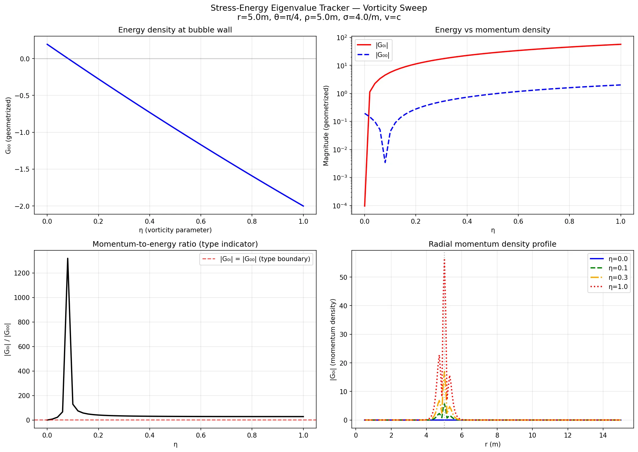 The vorticity cliff. Top left: energy density at the bubble wall drops from positive to deeply negative. Top right: momentum density (red) explodes while energy density (blue) barely changes. Bottom left: the momentum-to-energy ratio — the Type I/IV diagnostic — spikes above 1000 at η≈0.1. Bottom right: radial momentum profiles showing the flat blue line at η=0 (zero vorticity) versus the wild oscillations at η>0.
The transition happens at η = 0.018. Less than 2% vorticity. The momentum-to-energy ratio jumps from 0.0005 to 7.7 in that tiny window. Two eigenvalues form a complex conjugate pair — the definitive Type IV signature. The positive-energy ratio collapses from 1.25 to 0.63 at 5% vorticity, reaching 0.02 by 20%.
This isn’t a slope. It’s a cliff.
For engineering purposes, it means manufacturing tolerances below 1% on the curl-free condition. One percent. Whatever generates the warp field — if it has an engineering implementation, which is a big “if” — must maintain curl-free precision to a level comparable to semiconductor lithography. A vorticity contamination at the 2% level doesn’t degrade the solution. It destroys it.
The Trap
Finding the cliff was exciting. It suggested a path: if we could improve the energy conditions further — maybe even eliminate the remaining negative energy — we’d have something remarkable. The natural lever is the lapse function, α(r), which controls how fast time flows at each point in space. Every warp drive analysis before this assumed α=1 (uniform time flow). What if we let time flow slower inside the bubble?
I tried it. A sub-unit shell lapse, α ≈ 0.77 at the bubble wall, reduced the local NEC violation from -0.084 to -0.0012. A 68× improvement.
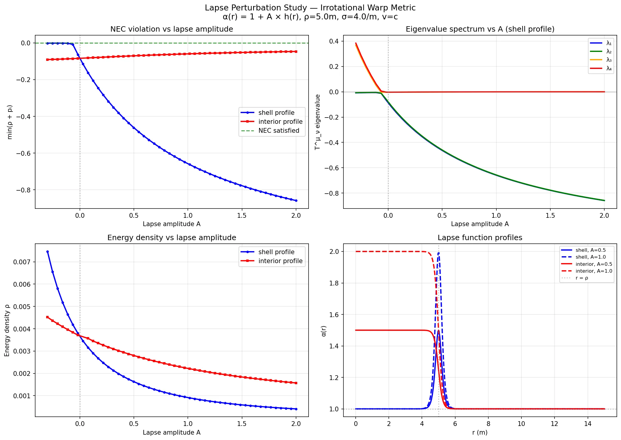 The lapse perturbation study. Top left: the shell profile (blue) shows dramatic NEC improvement near A=-0.23, approaching the green “NEC satisfied” line. The interior profile (red) barely responds. Top right: eigenvalue spectrum — two eigenvalues flip sign at A≈-0.23, explaining the local improvement. Bottom left: energy density drops sharply. Bottom right: the lapse profiles themselves.
Sixty-eight times better. At the bubble wall. I almost celebrated.
Then I integrated over the whole bubble.
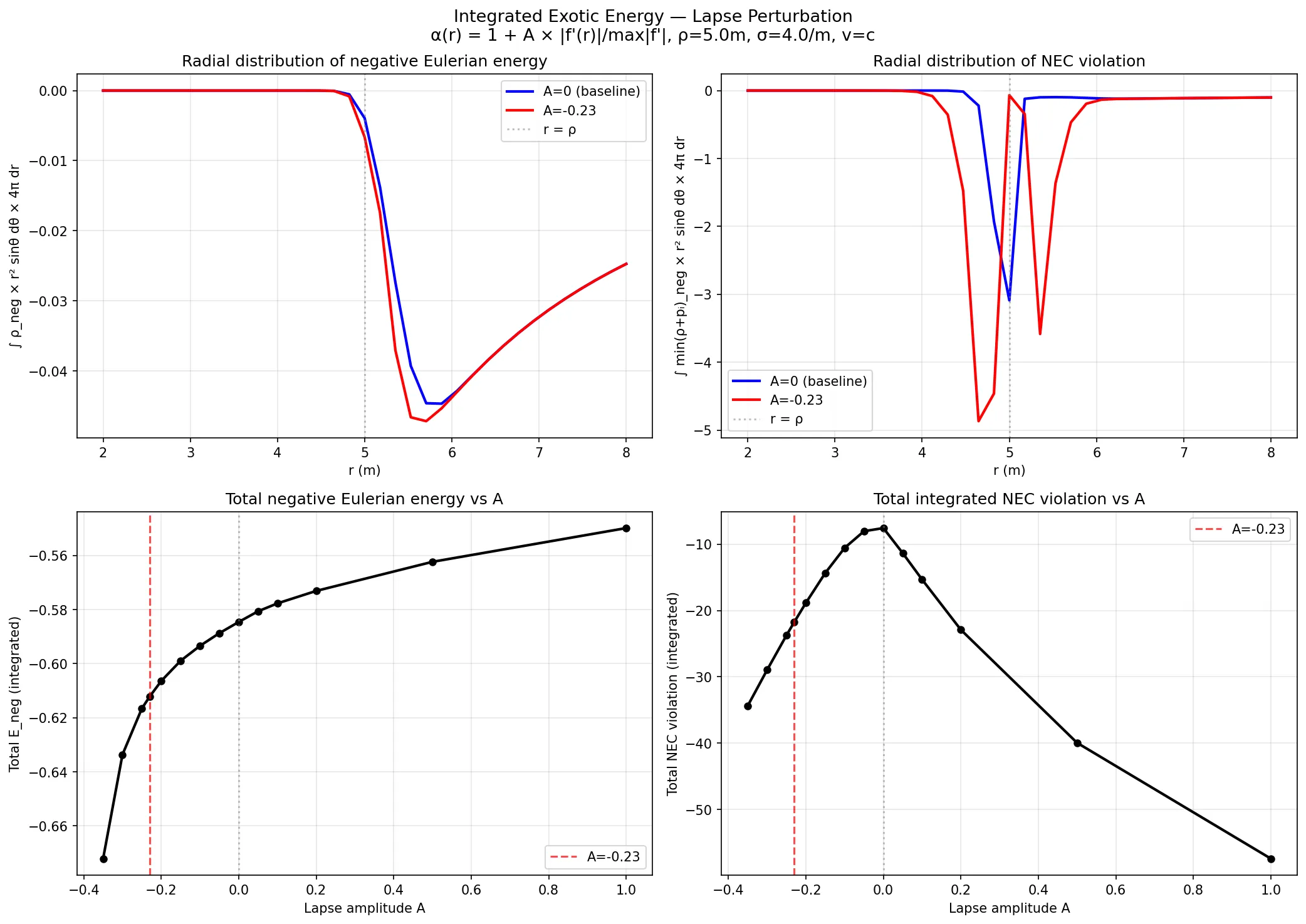 The integrated exotic energy tells a different story. Top left: the lapse moves the negative energy peak from the wall (r=5) to the inner shell (r≈4.7), but the total area under the curve doesn’t shrink. Top right: NEC violation distribution — the baseline (blue) concentrates at the wall, the optimized lapse (red) spreads it inward. Bottom row: total negative energy (left) and total NEC violation (right) versus lapse amplitude. The red dashed line marks A=-0.23, the “optimal” lapse. It’s not optimal at all — the total NEC violation is 2.9× worse.
The total integrated NEC violation is approximately lapse-invariant. The exotic energy that disappeared from the bubble wall reappeared at the inner shell. The lapse didn’t reduce the problem — it moved it. Like squeezing a balloon: press one side and the other side bulges.
This makes physical sense once you see it. The lapse is a foliation choice — it determines how you slice spacetime into spatial layers. Different slicings see the same total curvature content. You can’t eliminate curvature by choosing a different slicing any more than you can flatten a mountain by looking at it from a different angle.
Negative result #1: The lapse redistributes but does not reduce. The total exotic energy is a near-invariant.
The Mass Shell
If the lapse can’t help, what about spatial curvature? Instead of flat spatial slices (γ_ij = δ_ij), what about adding a real positive-mass shell around the bubble — curving space itself?
This is the approach Fuchs et al. (2024) used to build the first warp drive satisfying all energy conditions. They used the Warp Factory toolkit: non-unit lapse, non-flat spatial metric, subluminal velocity. The full ADM trifecta.
I tried the simplest version: a conformally flat spatial metric, γ_ij = ψ⁴(r) δ_ij, where ψ encodes the mass of a surrounding shell. The conformal factor satisfies the Hamiltonian constraint — in the nonlinear case, ∇²ψ = -2πρ₀ψ⁵. I solved this via parameter continuation in w = ln ψ variables, which tames the ψ⁵ blowup.
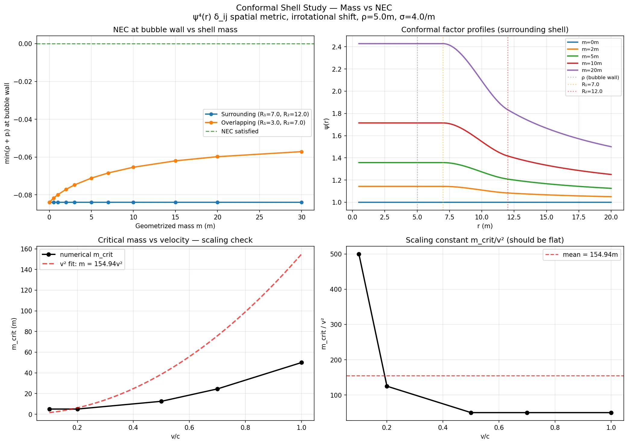 The conformal shell study. Top left: NEC at the bubble wall vs shell mass. The surrounding shell (blue) can’t see the wall at all — constant ψ inside = coordinate invariance. The overlapping shell (orange) improves NEC but never reaches zero. Top right: conformal factor profiles for different masses. Bottom row: critical mass scales as v² (left), with a roughly constant scaling factor (right, red dashed line).
Three more negative results:
Negative result #2: A mass shell outside the bubble has zero effect on the wall NEC. The interior conformal factor is constant — it’s a coordinate rescaling, not real curvature. The shell must overlap the bubble wall.
Negative result #3: Even with overlap, conformally flat spatial curvature saturates at about 30% NEC reduction. One scalar function ψ(r) can’t tune a 10-component tensor object. The NEC involves a 4×4 eigensystem; conformal flatness eliminates exactly the anisotropic degrees of freedom you’d need to satisfy it.
Positive result: The minimum shell mass scales as v² — confirmed numerically across two decades of velocity. This is the engineering curve. At v=0.01c (3,000 km/s, Alpha Centauri in 437 years), an irrotational warp drive needs roughly 5 Earth masses of shell material. At v=0.001c (galactic escape velocity), about 0.05 Earth masses.
The Advantage That Persists
Through all of this — the cliff, the lapse trap, the conformal saturation — one number held steady.
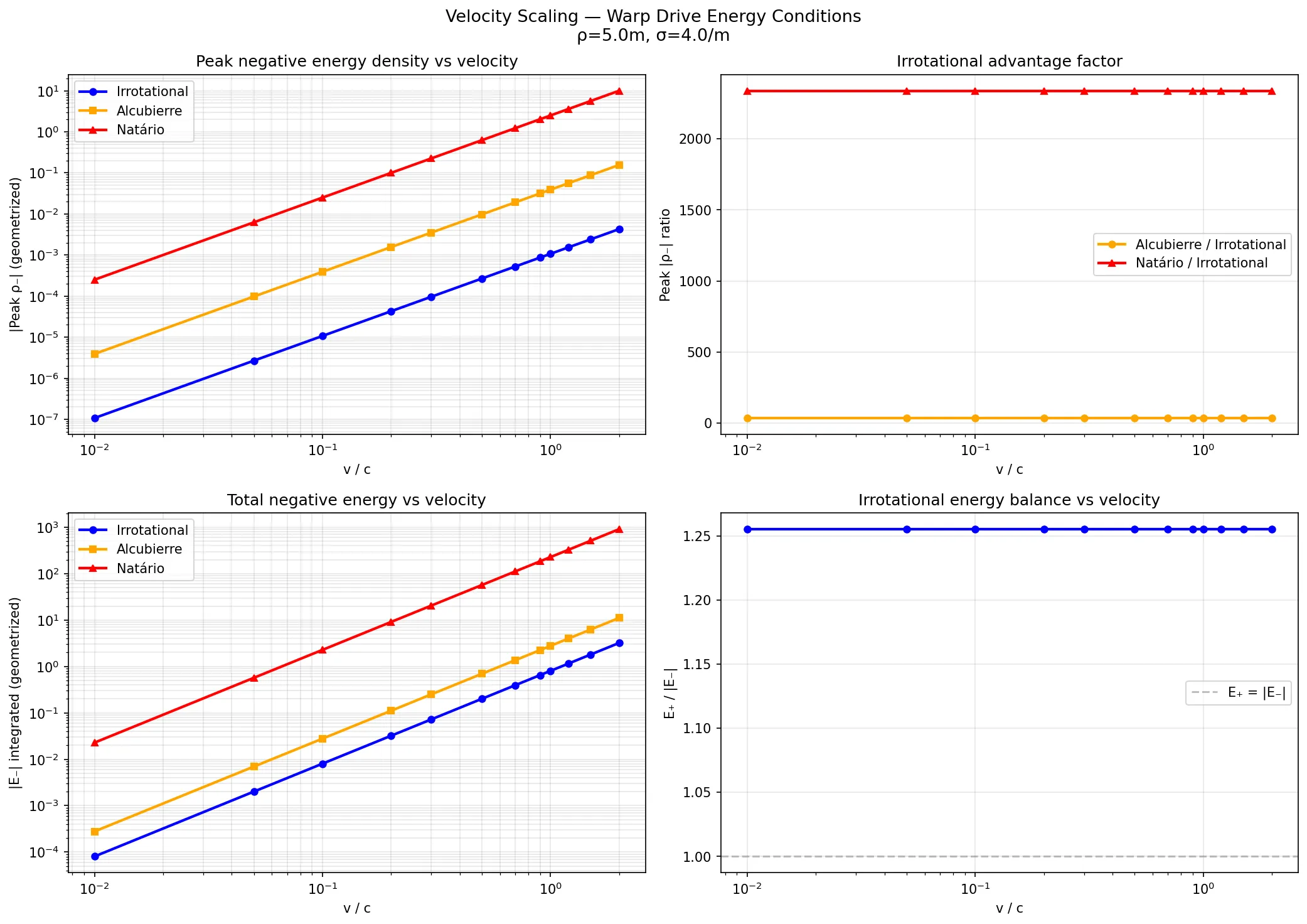 The irrotational advantage across velocities. Top left: peak negative energy density — the irrotational metric (blue) is consistently ~37× lower than the Alcubierre metric (orange) and ~2400× lower than Natário (red). Top right: these advantage factors are velocity-independent. Bottom left: total integrated negative energy shows the same separation. Bottom right: the energy balance E₊/|E₋| for the irrotational metric stays at 1.25 — more positive energy than negative — at all velocities.
The irrotational advantage — 37× lower peak negative energy density, 2400× lower energy ratio versus Natário — persists at every velocity from 0.01c to beyond light speed. It’s not a low-velocity artifact. It’s structural. The curl-free constraint on the shift vector fundamentally changes the topology of the stress-energy tensor, and that change doesn’t depend on how fast the bubble moves.
This means the irrotational advantage stacks with other improvements. Lower velocity (v² scaling), curved spatial slices (Fuchs approach), and irrotational shift all multiply. The design space isn’t a single optimization — it’s three independent levers.
The Revised Landscape
While running these computations, I found three recent papers that reshape the field:
Lentz is debunked. Celmaster & Rubin (2025) computed the full energy-momentum tensor for the Lentz “positive energy” warp geometry and found negative energy density regions. The flagship “no exotic matter” result from 2021 contained derivation errors. Even modified versions fail.
Metamaterials don’t work. Rodal himself (2025) showed that spatially varying gravitational coupling — the “metamaterial warp drive” idea — violates the contracted Bianchi identity. When made dynamical to fix conservation, it becomes a scalar-tensor theory ruled out by solar system tests to |γ-1| < 10⁻⁵.
De Sitter warp is impractical. Garattini & Zatrimaylov (2025) found positive-energy warp in expanding spacetime — but only at the cosmic expansion rate. About 70 km/s per megaparsec. Not useful for getting anywhere.
The shortcuts are gone. What survives:
| Approach | Status |
|---|---|
| Lentz geometry trick | Debunked (Celmaster 2025) |
| Metamaterial coupling | Debunked (Rodal 2025) |
| De Sitter embedding | Valid but impractical |
| Fuchs mass shell | Survives — all energy conditions satisfied |
| Rodal irrotational shift | Key ingredient — 37× reduction |
The field is narrowing to one viable path: real positive mass + irrotational shift + subluminal velocity. No geometry tricks. No metamaterials. No exotic matter. Just a very heavy, precisely engineered shell moving slower than light.
What I Learned
The hierarchy of optimization levers, from most to least effective:
- Spatial metric curvature (flat vs. curved γ_ij): potentially unlimited improvement — Fuchs achieved full energy condition satisfaction with non-flat slices
- Shift topology (irrotational vs. vortical): 37× in peak negative energy, hard phase boundary at 1.8% vorticity
- Geometry parameters (bubble size, wall steepness): ~100× range across the parameter space
- Lapse function alone: ~0× integrated improvement — redistributes but does not reduce
The negative results are the finding. You can’t fix a warp drive by adjusting the clock rate. You can’t fix it with a single conformal factor. You need the full spatial metric — six independent tensor components, not one scalar function — solved self-consistently with the shift and lapse through Einstein’s coupled constraint equations.
The 1.8% number stays with me. Not because it’s the most important result — the lapse invariance and the mass scaling matter more for engineering. But because it captures something about how physics works. The difference between a system that requires exotic matter and one that doesn’t — the difference between impossible and merely very difficult — lives in a 2% window of a single parameter.
Cliffs like that don’t show up unless the underlying structure is sharp. And sharp structure is where the physics lives.
All computations: brute-force finite differences on the full 4×4 Einstein tensor. Python, numpy, scipy, ~2 hours total CPU time. Seven source files, no machine learning, no GPU. Sometimes the interesting physics is in the structure, not the scale.